
Cap Rate Analysis: Apartments
Introduction
The Baseline Partners (BP) Portfolio Management (PM) Team analyzed capitalization rates and implied rates of investment return for four major types of commercial real estate (CRE) nationally and in five different regions over the period 2005-2021.The goal of the analysis was to understand the behavior of CRE valuations during the most recent several business cycles (including the credit crisis) and to gauge potential implications for CRE valuations in the current pandemic and post-pandemic cycle.
Definitions
The main data was downloaded from Bloomberg L.P. and consisted of Real Capital Analytics (RCA) capitalization rates broken down by geography and CRE asset type. The data series are divided into four asset types – Apartment, Office, Industrial, and Retail – and six regions: Northeast, South, Midwest, West, West Coastal, as well as the National aggregate. The data covers the period from January 2015 until April 2021 and includes a total of 196 monthly observations. According to RCA, the data point is the 12-month rolling average of capitalization rates based on independent reports of properties and portfolios over $10M in value. The data excludes refinancing transactions.
Capitalization rates were selected for this exercise because they (1) have been consistently aggregated over long periods of time by CRE vendors (such as RCA, CoStar, CBRE, Colliers, etc.) from a constant flow of appraisals, and (2) are readily available to external parties via the Bloomberg terminal. For a study on the behavior of CRE valuations like this, an alternative option would be to use CRE transaction-based price indices that use repeat-sales, comparable to the now-popular S&P CoreLogic Case-Shiller Home Price indices for the residential world. However, this option would require users to register for a particular service and rely on relatively sophisticated third-party aggregation techniques to draw conclusions.
But what is a capitalization rate or “cap rate”? A cap rate is the ratio between the net operating income (NOI) to the acquisition price (or value) of a particular property. The net operating income is the actual or anticipated net income that remains after all operating expenses are deducted from effective gross income (mostly rents) but before mortgage debt service and other non-operating expenses such as capital improvements to the building. Cap rates can be important inputs to real estate valuations and investment decisions because they help investors gauge the required rate of return of a given property and expectations of future rental income. At the same time, cap rates are a simple way of expressing and comparing property values, given a projected level of revenue/income (measured by the NOI), to other like-properties under similar market conditions. This approach is called direct capitalization.
When required rates of return are high and expected rental growth is weak, investors apply high cap rates when valuing properties because expected property cash flows are not likely to grow over time, , which imposes deeper discounts on future cash flows.
Discussion
Having collected the above data, BP’s PM team created a value index for each region and asset type combination and calculated four basic, univariate statistics from the historical monthly return series: mean, min, max and standard deviation. These statistics allow for a better understanding of the return distribution implied by changes in capitalization rates, and thus valuations, for different time windows (17 calendar years since 2005 and five multi-year holding periods described below). In addition, total holding period returns (HPR) were calculated over the same time windows to provide an idea of cumulative capital gains.
The selected time windows are meant to replicate reasonable holding periods:
1/2005 to 12/2009 (60 months): pre-credit crisis with disposition in the back end of the recession
1/2007 to 12/2011 (60 months): early credit crisis with disposition in early recovery stage
1/2010 to 12/2014 (60 months): early-stage recovery with disposition in mid recovery stage
1/2015 to 12/2019 (60 months): mid-stage recovery with disposition in late recovery stage
1/2005 to 4/2021 (196 months): full sample, inclusive of the COVID-19 pandemic
All returns presented in this analysis reflect only the gains from asset appreciation during a given period and do not include any returns from net cash flow (e.g. rental income). Including ongoing cash flow could change the return profile significantly for each asset class, but this is excluded here for simplicity and must be reserved for a future study.
Asset Type: Apartment
Returns on apartments ranged widely, between ‑19.6% and 22.5% (a 41.9% -spread) over the 2005 to 2021 sample period. The worst-performing year was, perhaps unsurprisingly, 2007, with apartments in the Northeast dropping 19.6% over the year. The best year for apartments was 2013, also in the Northeast region, with a 22.5% value appreciation over the year. The average annual (calendar) return over the 17-year period across the 5 regions was 1.70%, with the highest average annual performance in the West region at 2.30%. In terms of volatility, returns nationally saw an annualized volatility of 4.9% over the same period, with the most volatile region being the Northeast (19.4%) and the least volatile the South (6.5%).
The best holding period and geographic combination as an apartment investor would have produced a 41.0% return in the West Coastal region (CA, OR, WA) over the 2005 to 2021 window, the longest holding period available. The worst-performing window and geographic combination was between 2005 and 2009 in the Northeast, with a return of ‑18.6% . The spread in period returns over the five selected windows was 59.6%, illustrating the importance of timing. In this sample, avoiding 2007 would have produced an average pickup of 6.84% on the returns of an apartment portfolio.
Main takeaways:
For apartments, the worst-performing geography over the 17-year period was the Northeast, with a 4.0% HPR for the full period and a ‑18.6% return for 2005-2009, as mentioned above; the Northeast also had the highest annualized volatility of any region, at 19.4% for the full window
The best-performing investment window was the longest available (again, 17 years) in the West region, with a 41.0% holding period return (HPR) and a 2.3% average annual return
In the South, the average annual return over the 17-year period was 1. 9% and ranged between ‑9.8% and 10.0% over the same period, with a 6.5% annualized volatility
The Midwest, on the other hand, showed an average annual return of 1.8% and ranged between ‑11.0% and 18.0% over the same period, with a 12.4% annualized volatility
At the national level, the average annual return for apartments was 1.70%, with annualized volatility at 4.9%. The best-performing investment window was 2005 to 2021, with an HPR of 30.2%
Technical Appendix
In the direct capitalization method, we derive Market Value by dividing Net Operating Income (NOI) by Capitalization Rate. In our case, we have the Real Capital Analytics (RCA) capitalization rates, and we derive a value index through the formula below (assume a notional NOI of 1000):

Monthly returns (percent changes in the value of the above index) are calculated using the formula below:

We then annualized the monthly returns, using the standard calculation below:

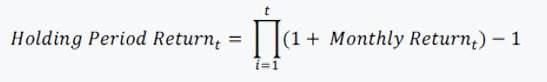
Holding period return (HPR) is the total return earned on an investment during the time that it has been held. In our case, holding period return is the return on $1 investment at time 0 compounded by the monthly return until time t. The HPR is calculate for the 5 hypothetical investment windows described on the Discussion section, as well as every calendar year from 2005 through 2021:
Volatility is a statistical measure of the dispersion of returns for a given security or market index. In our case, volatility is the standard deviation of the monthly returns. We have annualized the volatility of monthly returns using the standard calculation below:
